Combined Bayesian Classification

Finally, we constructed a third classifier as a combination of the two classifiers described above with the aim to achieve improved results, because, as we will show in the results, kNN and ID$3$ classifiers provide complementary information. This third classifier is based on the Bayes rule [43] estimation. When a new case is studied, it is classified according to the classic Bayes equation:

$$P(x\in B_c\vert A(x)) = \frac{P(A(x)\vert x\in B_c)P(B_c)}{\sum_{l=1..4}P(A(x)\vert x\in B_l)P(B_l)}$$ (3.6)

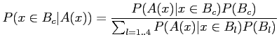
Translating this formula into words, we consider the probability of a mammogram $x$ , with set of features $A(x)$ , to belong to the class $B_c$ as the posterior probability. The prior is the probability of the mammogram to belong to a class before any observation of the mammogram. If there were the same number of cases for each class, the prior would be constant (for four categories, as is the case for BIRADS classification and hence $l=1..4$ , the constant value would be equal to $0.25$ ). Here we used as the prior probability the number of cases that exists in the database for each class, divided by the total number of cases. The likelihood estimation is calculated by using a non-parametric estimation, which is explained in the next paragraph. Finally, the evidence includes a normalization factor, needed to ensure that the sum of posteriors probabilities for each class is equal to one.

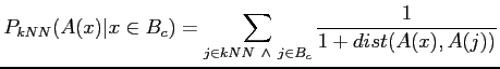
Combining the kNN and C$4.5$ classifiers is achieved by a soft-assign approach where binary (or discrete) classification results are transformed into continuous values which depict class membership. For the kNN classifier, the membership value of a class is proportional to the number of neighbours belonging to this class. The membership value for each class $B_c$ will be the sum of the inverse Euclidean distances between the $k$ neighbouring patterns belonging to that class and the unclassified pattern:

$$P_{kNN}(A(x)\vert x\in B_c)=\sum_{\substack{j\in kNN \wedge j\in B_c}} \frac{1}{1+dist(A(x),A(j))}$$ (3.7)

Note that with this definition, a final normalization to one over all the membership values is required. On the other hand, in the traditional C$4.5$ decision tree, a new pattern is classified by using the vote of the different classifiers weighted by their accuracy. Thus, in order to achieve a membership for each class, instead of considering the voting criteria we take into account the result of each classifier. Adding all the results for the same class and normalizing all the results, the membership for each class is finally obtained.