Both the ID![]() and C
and C![]() algorithms are based on the use of the
ID
algorithms are based on the use of the
ID![]() information criterion [43] to simultaneously
determine the best attribute to split on and at which threshold it
has to be split. This criterion is based on the information gain,
which measures how well a given attribute separates the training
examples according to their target classification at each step.
The main difference of both algorithms is that, while ID
information criterion [43] to simultaneously
determine the best attribute to split on and at which threshold it
has to be split. This criterion is based on the information gain,
which measures how well a given attribute separates the training
examples according to their target classification at each step.
The main difference of both algorithms is that, while ID![]() used
the information gain itself, C
used
the information gain itself, C![]() used the gain ratio.
used the gain ratio.
In our implementation, each leaf corresponds to a test ![]() of the
kind:
of the
kind:
![]() (feature
(feature ![]() is lesser or equal to the given
threshold
is lesser or equal to the given
threshold ![]() ). This test only has two possible outcomes: true or
false, and the issue is to find the best threshold to partition
the data. The splitting criterion used is the gain ratio.
). This test only has two possible outcomes: true or
false, and the issue is to find the best threshold to partition
the data. The splitting criterion used is the gain ratio.
The information gained by a test ![]() with
with ![]() outcomes is
defined by:
outcomes is
defined by:
where ![]() is the information associated with the
partitions over the set of patterns
is the information associated with the
partitions over the set of patterns ![]() (the database of
mammograms) and
(the database of
mammograms) and ![]() the entropy of the given partition, which
is defined below. Mathematically,
the entropy of the given partition, which
is defined below. Mathematically, ![]() is also defined by the
entropy:
is also defined by the
entropy:
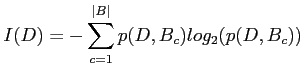
where ![]() is the probability that a
pattern/mammogram belongs to the
is the probability that a
pattern/mammogram belongs to the ![]() class (in this work,
class (in this work,
![]() , as there are four BIRADS classes). On the other hand,
, as there are four BIRADS classes). On the other hand,
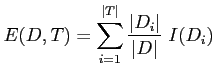
![]() refers to the entropy defined by the partition, which is
calculated as:
refers to the entropy defined by the partition, which is
calculated as:
where ![]() are the partitions of the data
are the partitions of the data ![]() defined
by the test
defined
by the test ![]() (the true and false instances). Thus, the
information gain is simply the expected reduction in entropy
caused by partitioning the examples according to an attribute.
This is the criterion used by the ID
(the true and false instances). Thus, the
information gain is simply the expected reduction in entropy
caused by partitioning the examples according to an attribute.
This is the criterion used by the ID![]() decision tree.
decision tree.
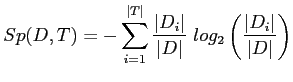
As the above criterion is maximal when there is one case in each
class, a new term is used to penalize this situation. Thus, the
split information (![]() ) is defined as the potential
information obtained by partitioning a set of cases and knowing
the class which a pattern falls in, and is given by:
) is defined as the potential
information obtained by partitioning a set of cases and knowing
the class which a pattern falls in, and is given by:
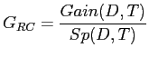
The gain ratio criterion ![]() used in the C
used in the C![]() decision tree is defined by:
decision tree is defined by:
This ratio is determined for every possible partition,
and the split that gives the maximum ![]() is selected.
is selected.
In order to obtain a more robust classifier, the boosting procedure described in [147] is used. The underlying idea of this machine-learning method is to combine simple classifiers to form an ensemble such that the performance of the simple ensemble member is improved. To achieve this, boosting assigns a weight to each instance of the training data, reflecting their importance. Adjusting these weights causes the learner to focus on different instances, leading to different classifiers. Thus, to construct the first decision tree, the weight of all the instances are initialized with the same value. Subsequently, the training data is classified by using this initial tree and an error rate is obtained, by counting the amount of misclassified data. Using this error rate, the weights are recalculated such that those belonging to misclassified instances are increased, and those belonging to correct classified instances are decreased. This process is repeated until either all instances are correctly classified or convergence is achieved. The final classification aggregates the learned classifiers by voting, where each classifier's vote is a function of its accuracy (the error rate).