The 2DPCA approach [194] is a recent improvement of the typical eigenfaces approach. As the authors argue 2DPCA has important advantages over PCA in two main aspects: firstly, it is simpler and more straightforward to use for image feature extraction since 2DPCA is directly based on the image matrix, and secondly, it is easier to accurately evaluate the covariance matrix5.2.
In the original eigenfaces approach, each image of size
![]() is transformed into a vector of size
is transformed into a vector of size ![]() , in contrast to
the natural way to deal with two dimensional data, which would be
treating it as a matrix. This is the motivation of
2DPCA [194].
, in contrast to
the natural way to deal with two dimensional data, which would be
treating it as a matrix. This is the motivation of
2DPCA [194].
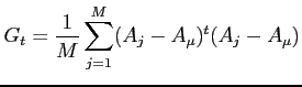
The algorithm starts with a database of M training images. The
image covariance matrix ![]() is calculated by:
is calculated by:
where ![]() is the mean image of all training samples.
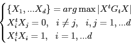
Then, using the Karhunen-Loeve transform it is possible to obtain
the corresponding face space, which is the subspace defined as:
is the mean image of all training samples.
Then, using the Karhunen-Loeve transform it is possible to obtain
the corresponding face space, which is the subspace defined as:
where X is a unitary column vector. The first equation
looks for the set of ![]() unitary vectors where the total scatter
of the projecting samples is maximized (the orthonormal
eigenvectors of
unitary vectors where the total scatter
of the projecting samples is maximized (the orthonormal
eigenvectors of ![]() corresponding to the first
corresponding to the first ![]() largest
eigenvalues). On the other hand, the other two equations are
needed to ensure orthonormal constraints.
largest
eigenvalues). On the other hand, the other two equations are
needed to ensure orthonormal constraints.
With the selected set of eigenvectors it is possible to construct
a family of feature vectors for each image. Thus, for an image
sample ![]() , the projected feature vectors (the principal
components)
, the projected feature vectors (the principal
components)
![]() are found by:
are found by:
| (5.3) |
It is important to note that while for PCA each principal
component is a scalar, for 2DPCA each principal component is a
vector. It is this set of vectors for image that is used to
construct the feature image (a matrix of size
![]() )
referred to as
)
referred to as
![]() .
.
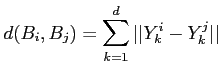
In a similar way to the eigenfaces approach, comparing images means to compare the constructed features. As the dimension of the feature space has increased in one dimension, now the comparison of images is done by comparing matrices:
where
![]() denotes the Euclidean distance
between the two principal component (vectors)
denotes the Euclidean distance
between the two principal component (vectors) ![]() and
and ![]() .
To obtain an
.
To obtain an ![]() value we adopt the analogous probabilistic
scheme described in Section
value we adopt the analogous probabilistic
scheme described in Section ![]() .
.