The first objective of the proposal is the construction of a
general mass template, which should take the shape variations into
account. The main aim is that pixels with a boundary morphology
which has a major representation in the database have a higher
probability than the rest of the pixels. Hence, as the template is
represented as an image, the pixel brightness will be associated
with the probability of belonging to a contour. Thus, the designed
template will have intensity 0
for those pixels which certainly
do not represent a contour, intensity ![]() for the pixels which in
all images of the database are on a contour (if any), and
intermediate values for the rest of the pixels.
for the pixels which in
all images of the database are on a contour (if any), and
intermediate values for the rest of the pixels.
An initial solution for the construction of this template consists
in considering only the boundaries of manually segmented masses.
Note, however, that this solution prefixes a set of contours, and
contours different to them will probably be refused while, in
contrast, the probability to find two masses with similar shape is
very low. Thus, in order to obtain a more general template, it is
constructed by looking for the sub-space that these boundaries
define. This is achieved by adapting the eigenfaces approach
described in Section ![]() . Moreover, using this
approach only a rough manual segmentation is needed, just
including the centre and size of the mass.
. Moreover, using this
approach only a rough manual segmentation is needed, just
including the centre and size of the mass.
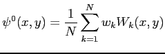
With the obtained eigenmasses, it is possible to construct a
probabilistic template per size (note from the previous section
that the masses have been clustered according to their size and
different templates can be created). For constructing these
templates, the ![]() eigenvectors containing
eigenvectors containing ![]() of variation
explanation were used, considering more probable shapes those with
the greatest eigenvalue. Therefore, an initial template is
constructed as :
of variation
explanation were used, considering more probable shapes those with
the greatest eigenvalue. Therefore, an initial template is
constructed as :
 |
(4.3) |
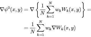
where
![]() is the template,
is the template, ![]() is the
is the
![]() -th eigenmass and
-th eigenmass and ![]() its normalized eigenvalue (the
corresponding eigenvalue divided by their sum). The contour of the
eigenmasses is found by extracting the gradient from
its normalized eigenvalue (the
corresponding eigenvalue divided by their sum). The contour of the
eigenmasses is found by extracting the gradient from
![]() :
:
 |
(4.4) |
This equation (image) represents the template as a weighted contours of the eigenmasses. In order to obtain a deformable template, it is necessary to specify the modes of deformation of such initial (rigid) template. Note that the object deformation in an image is an unknown parameter of the model which will be estimated during the template matching step.
Plausible shapes are those obtained from linear combinations of
the eigenmass contours, and deformation will only affect the
weight of the eigenvalues of each eigenmass. This is represented
by a vector ![]() of size N:
of size N:
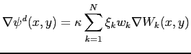 |
(4.5) |
where
![]() is the deformed template and
is the deformed template and
![]() is just a normalization factor. With this definition, the
vector
is just a normalization factor. With this definition, the
vector ![]() is all ones when no variations from the template
occur, and results in larger difference to the original template
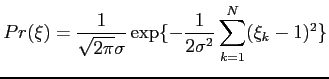
as it increases/decreases its values. Hence, assuming a Gaussian
distribution, the probability of finding a template with such
deformation is:
is all ones when no variations from the template
occur, and results in larger difference to the original template
as it increases/decreases its values. Hence, assuming a Gaussian
distribution, the probability of finding a template with such
deformation is:
Note that with this definition a new parameter (![]() ) is
included. Changes in the value of
) is
included. Changes in the value of ![]() represent a more rigid
(small
represent a more rigid
(small ![]() ) or a more flexible (large
) or a more flexible (large ![]() ) template.
Figure
) template.
Figure ![]() shows the templates for four
classes representing the range of mass sizes in the database.
shows the templates for four
classes representing the range of mass sizes in the database.
|
Moreover, Figure ![]() shows the average
intensity over a circle (y-axis) as a function of the radii to the
mass centre (x-axis), detailed for each of the four sizes. The
peak in each curve represents the radii with highest probability
of being a contour of a mass. Note that larger templates are not
only a translation of the smaller ones at different radii but also
have a different profile, showing the need of having a different
training set for each size.
shows the average
intensity over a circle (y-axis) as a function of the radii to the
mass centre (x-axis), detailed for each of the four sizes. The
peak in each curve represents the radii with highest probability
of being a contour of a mass. Note that larger templates are not
only a translation of the smaller ones at different radii but also
have a different profile, showing the need of having a different
training set for each size.
![\includegraphics[height=7 cm]{images/templatesProfile.eps}](img572.png)
|
![\includegraphics[height=1.75 cm]{images/template1.eps}](img568.png)
![\includegraphics[height=2.35 cm]{images/template2.eps}](img569.png)
![\includegraphics[height=3 cm]{images/template3.eps}](img570.png)
![\includegraphics[height=3.75 cm]{images/template4.eps}](img571.png)